Fig. 2: A model of a 4 qubits processor implementing the time-dependent Hamiltonian

Fig. 2: A model of a 4 qubits processor implementing the time-dependent Hamiltonian
Here the time-dependent transverse magnetic fields {hti(t)} on each qubit drive the system in excited states. sigmai{x,z} are Pauli matrices for the i-th qubit, hi are on-site local magnetic fields and J{ij} are pairwise couplings between the qubits.
The many-qubit basis, i.e. the computational basis, is denoted by 4 labels, indicating
the state of each qubit by 1 for spin up or 0 for spin down:
which are eigenstates of the Ising Hamiltonian. The diagonal matrix elements of the
Ising Hamiltonian are:
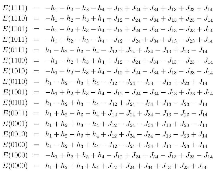
Thus we have a 16 X 16 matrix to diagonalize to get the eigenenergies of the 4 qubit
system.
Non-zero off-diagonal matrix elements of the interaction Hamiltonian exist only between computational basis states differing by a single label, i.e. by the flip of a single spin, for instance:
At t=0 the effect of {hti(t=0) not equal 0} is to mix in all computational basis states leading to the ground state of the 4 qubit system perturbed by the transverse magnetic fields. As {hti(t) -> 0} with time the time-dependent ground state changes. At the annealing time t=tf the external local transverse magnetic fields are switched off, i.e. {hti(tf)= 0} and the 4 qubit system is the solution of the Ising hamiltonian. A time development with crossing of eigenstates provides two distinct possibilities. The change will be adiabatic if {hti(t)} change slowly with time, leaving the system in the adiabatic time-dependent ground state. If {hti(t)} change fast with time the 4 qubit system may develop diabatically with time, i.e. it may stay on the potential curve of an excited eigenstate.
It is our aim to evaluate the probabilities for the adiabatic and diabatic development of the 4 qubit system in the time-dependent external local transverse magnetic fields {hti(t)}. To this purpose we have to test what is the meaning of slow and fast switching on of the local transverse magnetic fields.
The first task is to get the crossing states as lowest energy states so that the adiabatic development by extremely slow switching on of the transverse magnetic fields (tmf) {hti} leaves the system on the lowest energy curve, which changes its character with the time variations of {hti(t)}. This is the global minimum state, which is a superposition of eigenstates of the non-perturbed (by {hti(t)}) system. A fast switching on of the {hti}'s may lead to the diabatic development, i.e. the system remains in an excited eigenstate of the 4 qubit system which it higher in energy compared to the global minimum state.
First attemps led to two energetically low lying crossing states, however they were
not the energetically lowest lying states of the system. The plot refers to the
development of the eigenstates when the local transverse magnetic fields are
switched on very slowly so that the system develops adiabatically.
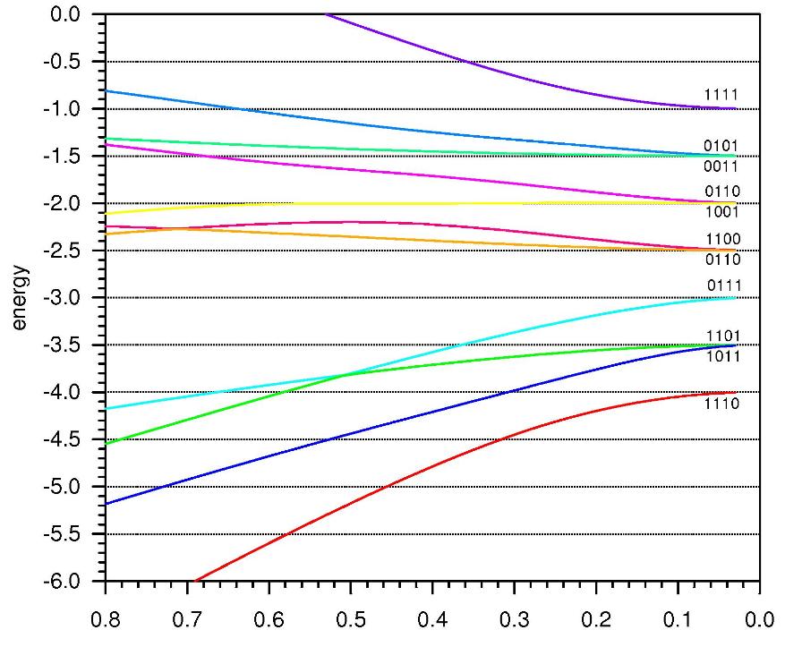
Fig. 3: Eigenstates of the 4 qubits model in interaction with the local transverse magnetic fields as a function of the magnitude of {ht1}. The local transverse magnetic fields are switched on slowly so that the system develops adiabatically into the global ground state.
The crossing is between eigenstates with dominating contribution from the basis states |0111> and |1101>.
Manipulations with the values of hi and J14 lead to shifting these states to lower
energies and to their avoided crossing in the limit of adiabatic development,
as it is shown in fig. 4.
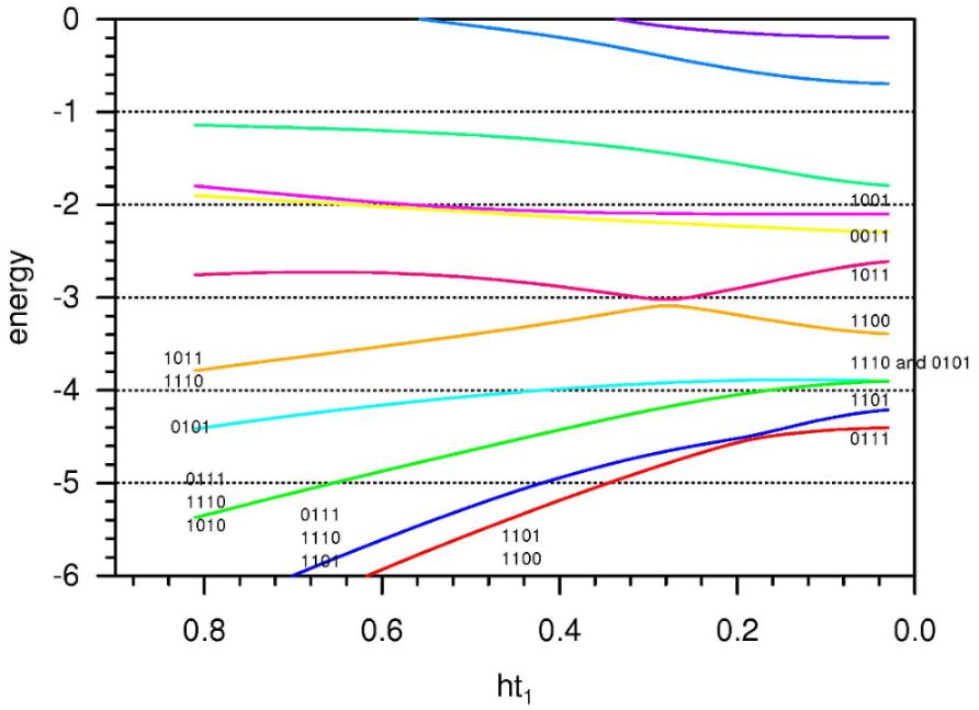
Fig.4: As in fig. 3 The parameter choice can be seen in the upper right corner and
leads to a non-zero minimal energy gap at the avoided crossing between the two
lowest energy eigenstates.
The occupation of the states with spin 1 on the third qubit, which will be shown in fig. 5 as a function of time, shows the adiabatic development of the system without a spin flip.
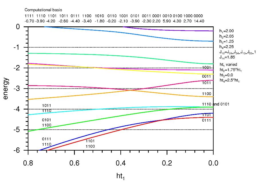
Fig.5: As in fig. 3. The parameter choice can be seen in the upper right corner. It differs from the parameters in fig. 4 by the choice of ht3=0. The gap beteen the global minimum state and the first excited state is reduced to zero.
It is possible to reduce the gap by reducing the value of ht3 which leads to shifting up of the eigenenergy of the state with main component |0111> due to its weakend interaction with the higher lying |0101> (cf. fig. 5). An alternative is to increase ht4 which leads to energy lowering of the eigenstate with main component |1101> due to its interaction with the basis state |1100> shown in fig. 7.
The energy differences between the first two excited states and the global minimum state is plotted in fig. 6 as a function of the transverse magnetic field ht1 is nearly zero. This presents a problem for the competition between diabatic and adiabatic time developmenmt of the system, therefore we revert to the parameters leading to a somewhat larger minimal energy gap at the time of avoided crossing (cf. fig. 7).
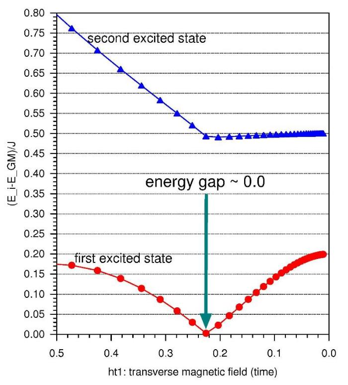
Fig. 6: Energies of the first two excited states of the 4 qubit system relative to
the global minimum state as a function of the transverse local magnetic field
ht1. The minimum gap between the global minimum state and the first excited state
is reduced nearly to zero at the time of avoided crossing.
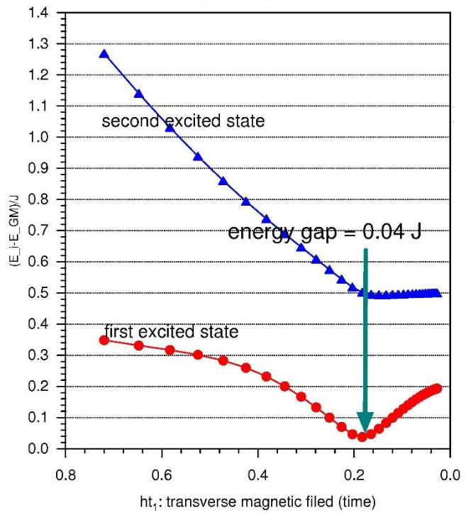
Fig. 7: As in fig. 7 with different parameter choice. The minimum gap between the
global minimum state and the first excited state is 0.04J12.
We assign the variations of the local and transverse magnetic fields to variations with time. Therefore we have to solve the time-dependent Schrödinger equation with a time dependent Hamiltonian:
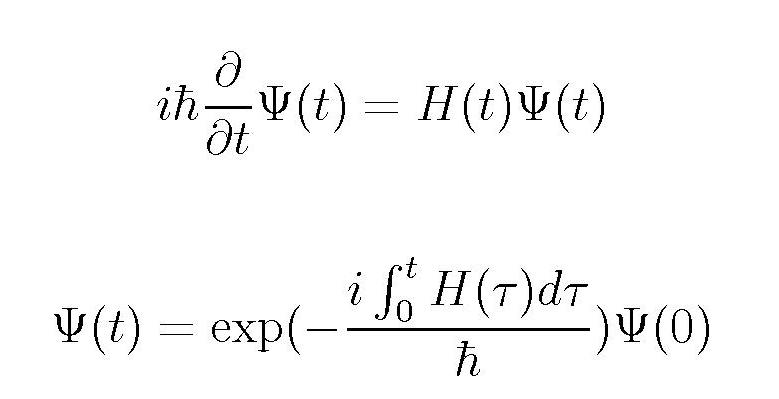
For the solution we need the eigenvalues of H(t) at time t. To get them we need the values of {hi} and V(t), i.e. of {hi(t)} and {hti(t)} at time t.
The development with time of the eigensolutions of the time dependent Hamiltonian (no phonons, no gravitons) is is shown in fig. 8. The parameters are those used for the plots in figs. 4 and 7.
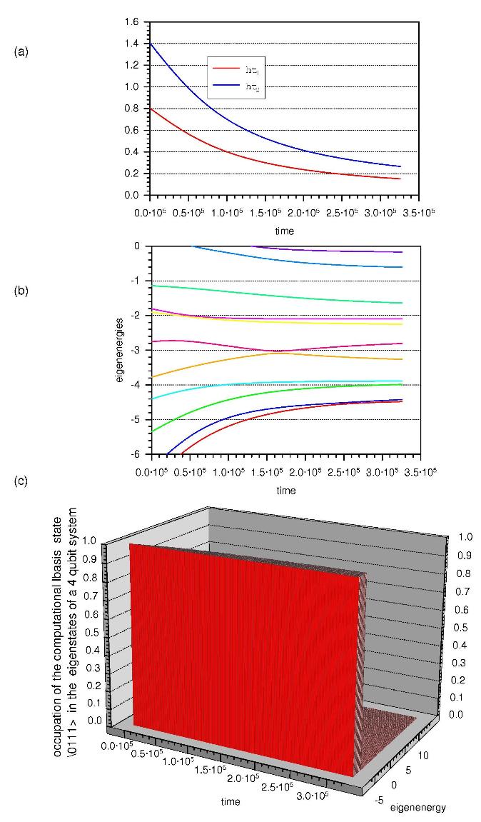
Fig. 8: (a) Variation with time of the transverse magnetic fields. In the uppermost
plot only ht1(t) and ht2(t) are shown. (b) The plot in the middle shows the variation
with time of the lowest eigenenergies. (c) The development with time of the occupation
of the 4 qubit state, corresponding to the global energy minimum state at the final
time t=tf, is shown in the lower plot. The quantity plotted is the modulus
squared of the coefficient with which the computational basis state |0111> participates
in all eigenstates as a function of time.
The 4 qubit state at time t=tf, when the local and transverse magnetic fields are
switched off,
corresponding to the global energy minimum, is the computational state |0111>. Starting
with an initial state, the lowest eigenstate for the system with non-zero values
of the magnetic fields at t=0, which is a superposition of all compuational basis
states, the 4 qubit system develops adiabatically with time, staying on the lowest
energy curve upon reducing the external local and transverse magnetic fields.
This is obvious in the lowest panel of fig. , where the distribution of the modulus
squared of the coefficient with which the computational basis state |0111> over
all eigenstates is plotted as a function of time. At all times from t=0 to t=tf
the system is in the global energy minimum state which is dominated by the basis
state |0111>. We refer to this development of the 4 qubit system as slow development
with time in contrast with the fast development described in the next section.